Basic K-means algorithm in GNU Octave

Months ago I started to read “Introduction to Applied Linear Algebra - Vectors, Matrices, and Least Squares” by Stephen Boyd and Lieven Vandenberghe (link). It is a beginner-friendly book. It can be downloaded for free, and there is a lot of additional material, including videos from Stephen Boyd’s lectures.

In the book, they show very early how simple linear algebra tools can be useful. Chapter 4 is about clustering, and they use the K-means algorithm as an example. The algorithm is built on top of very simple ideas, so it is surprising how good its results can be.

Here, I take a look at the K-means algorithm following the explanation from the book and show a basic implementation. I will use GNU Octave, which is what I was using for examples and exercises from the book.

How clustering works

The problem is to group observations into

k

clusters based on their similarity. The idea is to take each vector, check how similar it is to each group, and assign it to the closest group. But what defines a group? Well, a group representative, a vector that ‘summarizes’ all the vectors in the group. However, when you assign a new vector to a group, the group representative may change! And then the similarities change, and vectors may need to be re-assigned. So it is a circular problem.

An optimal solution for this problem is almost impossible, but suboptimal clustering can be done, and it works pretty well. To solve this problem, K-means is only one of many clustering algorithms available.

Measuring how good a clustering is

We need to define the objective function to be optimized. This function produces a single number that tells how well the algorithm is doing, and allows us to compare different clustering approaches.

However, before that, we need to pick a measure of similarity between vectors. I use the Euclidean distance, which is the one used in the book. It is defined as the norm of the difference between vectors:

Note: the code uses squared distance to avoid computing the square root. The result is not altered by this.

Ok, now the objective function. Suppose that we have

N

n

-vectors. We define

J

as:

where

x_{i}

is the

i

-th vector and

z_{ci}

its group representative. This is the within-cluster sum of squares (WCSS). When vectors are close to their group representatives,

J

is small, so we want to minimize

J

J

depends on two things: the assignment of vectors to groups, and the group representatives. The procedure to select them is the clustering algorithm.

The K-means algorithm

Convergence

Each iteration can only make

J

smaller or keep it the same: assigning each vector to its closest representative cannot increase

J

, and setting each representative to the mean of its group cannot increase it either, because the mean is exactly the vector that minimizes the sum of squared distances within the group. Since there is a finite number of possible group assignments, the algorithm eventually stops changing. That is what “repeat until convergence” means in the algorithm above.

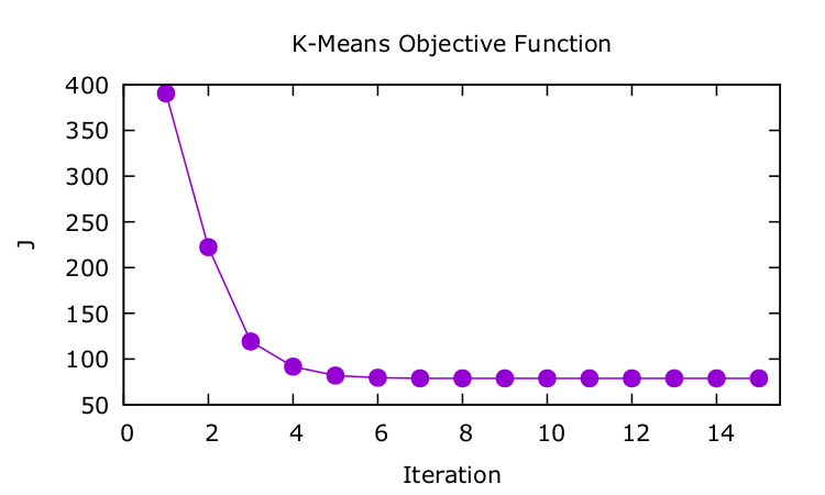
A real implementation would stop when the assignments no longer change between iterations. Here, I don’t check for convergence: I just run a fixed number of iterations (max_iter = 15, line 10 in code), which is enough for this problem, as the plot of

J

shows.

Example in GNU Octave with the iris dataset

The iris dataset has data from three different species. It is not a hard problem to separate them, and since the idea was to implement the algorithm by hand, it was a simple dataset to use.

In the first run, group representatives (

z

vectors) need to be created. The simplest (but not optimal) method is to pick a random vector from the dataset for each group (function init_random_z, line 25). Then the algorithm will run in a loop. Here I set a maximum number of iterations to 15.

The algorithm starts with step 1: assign vectors to groups. For each vector, it computes the distance to all the group representatives, and assigns it to the closest group (assign_class, line 40).

After all vectors have been assigned to a group, it goes into step 2: update group representatives. For each group, it picks all the vectors assigned to that group and averages them (update_centroids, line 60). That will be the new group representative for that group.

Before starting a new iteration, the algorithm computes

J

using the objective function presented above (compute_j, line 13). This value is stored to be plotted later.

These three functions, assign_class, update_centroids and compute_j, run 15 times (the max number of iterations I used). At the end, the vector

c

is returned. That is, the vector that says to which group each observation belongs.

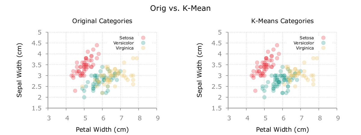
Here is a plot comparing the real species and the ones predicted by this basic K-means implementation:

The result is pretty good! Of course the simplicity of the dataset helps, but still it is surprising how such a simple method can produce useful information.

Finally, here is a plot of

J

during each of the 15 iterations. See how the value drops during the first iterations and then remains almost constant.

Code

     1  % Clustering with K-means
     2  
     3  % Load the data
     4  data = load("data/iris.txt");
     5  
     6  X = data(:, 1:4);
     7  y = data(:, 5);
     8  
     9  k = 3;
    10  max_iter = 15;
    11  
    12  
    13  function j = compute_j(X, c, z) 
    14    n = size(X, 1);
    15    j = 0;
    16    for i = 1:n
    17      c_i = c(i, :);
    18      x_i = X(i, :)';
    19      z_j = z(c_i, :)';
    20      j = j + ((x_i - z_j)' * (x_i - z_j));
    21    endfor
    22  endfunction
    23  
    24  
    25  function z = init_random_z (X, k)
    26    n = size(X, 1);
    27    z = zeros(k, size(X, 2));
    28    for i = 1:k
    29      random_i = randi(n);
    30      z(i, :) = X(random_i, :);
    31    endfor
    32  endfunction
    33  
    34  
    35  function d = square_dist (a, b)
    36    d = ((a-b)'*(a-b));
    37  endfunction
    38  
    39  
    40  function new_c = assign_class (X, z)
    41    n = size(X, 1);
    42    k = size(z, 1);
    43    new_c = ones(n, 1);
    44  
    45    for i = 1:n
    46      dist = zeros(k, 1);  % distances from the ith vector to the centroids
    47      x_i = X(i, :)';
    48  
    49      for j = 1:k
    50        z_j = z(j, :)';
    51        dist(j, 1) = square_dist(x_i, z_j);
    52      endfor
    53  
    54      [~, min_i] = min(dist);
    55      new_c(i, 1) = min_i;
    56    endfor
    57  endfunction
    58  
    59  
    60  function z = update_centroids(X, c, k)
    61    z = init_random_z(X, k);
    62    for j = 1:k
    63      x = X(c == j, :);
    64      if (size(x, 1) > 0)
    65        z(j, :) = mean(x);
    66      endif
    67    endfor
    68  endfunction
    69  
    70  
    71  function [y_hat, j_history] = kmeans(X, k, max_iter)
    72    n = size(X, 1);
    73  
    74    z = init_random_z(X, k);
    75    c = ones(n, 1);
    76  
    77    y_hat = c;
    78    j_history = zeros(max_iter, 2);
    79  
    80    for i = 1:max_iter
    81      c = assign_class(X, z);
    82      z = update_centroids(X, c, k);
    83      j_history(i, :) = [i, compute_j(X, c, z)];
    84    endfor
    85  
    86    y_hat = c;
    87  endfunction
    88  
    89  
    90  [y_hat, j_history] = kmeans(X, k, max_iter);
    91  
    92  
    93  dlmwrite("data/outputs/classified.dat", [data, y_hat], "delimiter", " ", "precision", "%.3f");
    94  dlmwrite("data/outputs/j_history.dat", j_history, "delimiter", " ", "precision", '%.3f');