Notes on Variance Inflation Factor (VIF)

Published: 2026-09-01

Some statistical models and machine learning algorithms perform poorly when predictor variables are highly correlated. Having multiple predictors that are linearly dependen is known as multicollinearity.

A well-known tool to check for multicollinearity is the variance inflation factor (VIF). My first encounter with the VIF was reading Graham’s (2003) paper¹, probably not the best choice for an introduction to the topic (Oh boy, Figure 1 was hell).

After that painful first contact, I ran into the VIF a lot when doing data analysis. The rule of thumb says that a variable should be dropped if it has a VIF > 10. Ok, got it. But what does a high VIF mean?

Here, I walk through the basics of the VIF to gain some intuition. I will not dive into how it affects modelling, but just look at what the VIF is, how it is computed and what it represents.

But what is the VIF?

For now, let’s skip why collinearity inflates the variance of the estimated coefficients (that may be another post). With that fact accepted, we can take a look at the definition from Wikipedia:

“The VIF provides an index that measures how much the variance of an estimated regression coefficient is increased because of collinearity.”

So, if you put highly correlated variables in the model, you get imprecise estimates. Real effects may end up looking non-significant.

The VIF is a term that multiplies the variance of the estimator:

$$VIF_{i} = \frac{1}{1 - R_{i}^2}$$

Here, $i$ represents the $i$-th predictor variable. The good part is the $R_{i}^2$. This is the coefficient of determination obtained by regressing the $i$-th variable on the rest of the variables. Therefore, when a variable is largely explained by the other variables, you get a high $R^2$, which results in a high VIF.

How it is implemented: example from the usdm package

To check that the VIF is really that simple, I looked at the code from the usdm package to see how they implement it in R. The following code is the internal function that handles the VIF in usdm::vif.R:

.vif <- function(.dd) {
  z<-rep(NA,ncol(.dd))
  names(z) <- colnames(.dd)
  for (i in 1:ncol(.dd)) {
    z[i] <-  1 / (1 - summary(lm(.dd[,i]~.,data=.dd[-i]))$r.squared)
  }
  return(z)
}

Here, .dd is a data frame. The function allocates space to store one value for each column from .dd, names that vector with the column names and, then iterates over each column and runs a linear model: lm(.dd[,i]~.,data=.dd[-i]).

This model is a regression with the $i$-th column as response and all the other columns as predictors (expressed with ~.). Then it takes the summary for that model and extracts the $R^2$. Finally, it computes the $1 / (1 - R^2)$.

Computing the VIF by hand with the iris dataset

Let’s compute the VIF for the variables from the iris dataset, which is available by default on R. Take the numeric columns from iris:

X <- iris[ , 1:4]
head(X)
##   Sepal.Length Sepal.Width Petal.Length Petal.Width
## 1          5.1         3.5          1.4         0.2
## 2          4.9         3.0          1.4         0.2
## 3          4.7         3.2          1.3         0.2
## 4          4.6         3.1          1.5         0.2
## 5          5.0         3.6          1.4         0.2
## 6          5.4         3.9          1.7         0.4

First, a look at the results from usdm::vif().

usdm::vif(X)
##      Variables       VIF
## 1 Sepal.Length  7.072722
## 2  Sepal.Width  2.100872
## 3 Petal.Length 31.261498
## 4  Petal.Width 16.090175

The VIF for Petal.Length is extremely high. Let’s reproduce that one ‘by hand’.

Write a linear model with Petal.Length as the response, and the rest as predictors:

res <- lm(Petal.Length ~ Sepal.Length + Sepal.Width + Petal.Width, data = X)
summary(res)$r.squared
## [1] 0.9680118

Then the VIF can be computed:

r2 <- summary(res)$r.squared
1 / (1 - r2)
## [1] 31.2615

This is the same output produced by usdm::vif().

The link between VIF and $R^2$

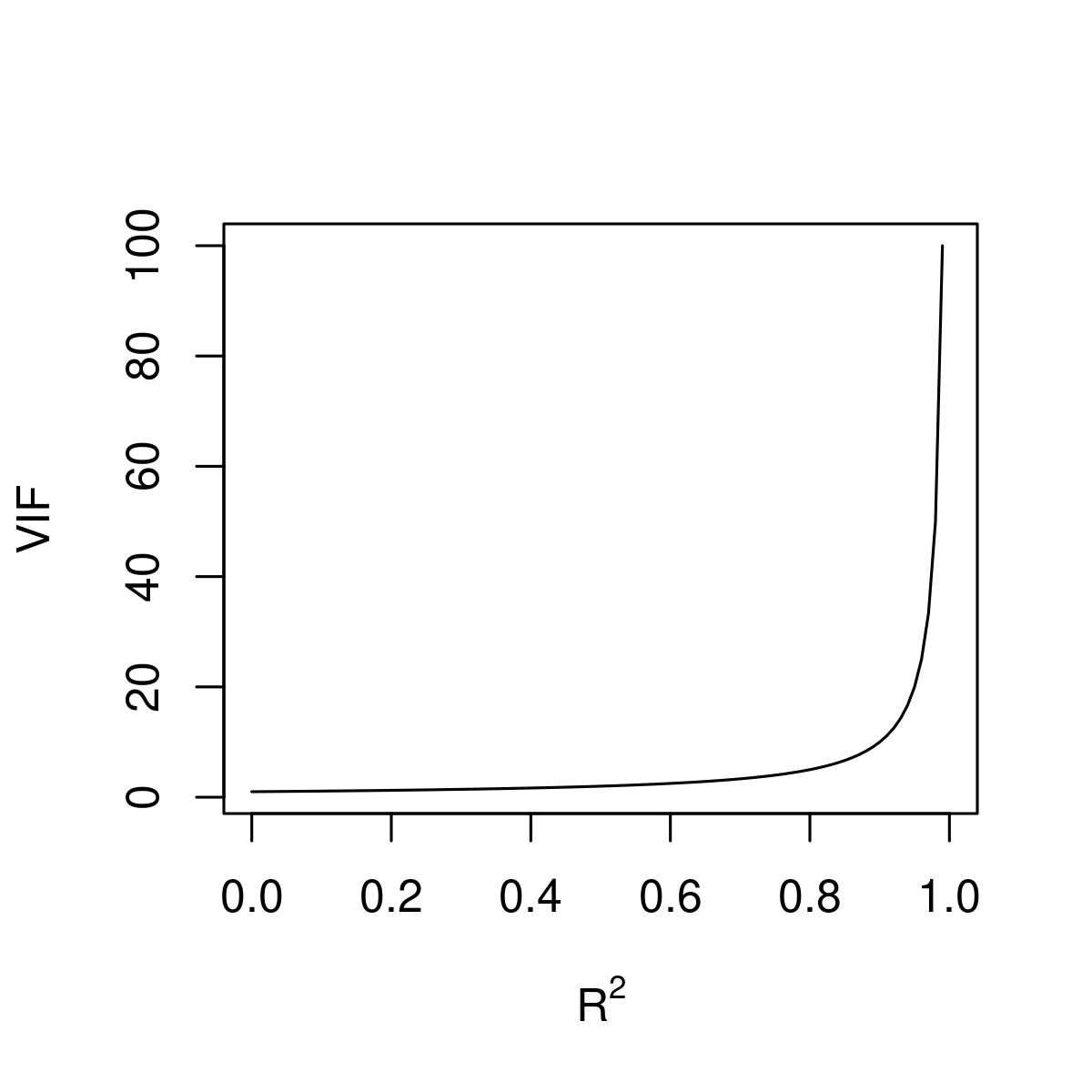
Going back to that rule of dropping a variable when VIF > 10, what $R^2$ does that threshold correspond to? Well, an extremely high $R^2$: 0.9!

1 / (1 - 0.9)
## [1] 10

To get an idea, this is how VIF and $R^2$ are related:

my_vif <- function(x) { 1 / (1 - x) }
rs <- seq(from=0, to=1, by=0.01)
plot(rs, my_vif(rs), xlab=expression('R'^2), ylab="VIF", type="l")

Final thoughts

Here I only looked at the VIF and not at the multicollinearity problem. In fact, I didn’t dig into what an inflated variance in practice. I just wanted to have some intuition about the VIF and what was going on behind that number.

• A VIF > 10 corresponds to an $R^2$ of 0.9, which is crazy.

• For VIF > 30 ($R^2$ ~ 0.97!), you can almost write the variable as a linear combination of the others. It does not provide any new information to the model.

• The R package car also implements generalized variance inflation factor (GVIF)², which is a bit more complex. It runs on models and not on datasets, but for a linear model with only numeric predictors it is the same as the VIF shown above.